Paul Khuong mostly on Lisp

This is a follow-up to an earlier post from April 2009 that has been mostly ready for almost one year now, so some of the details in the numerical results may be a bit foggy.

As I wrote back back in January, Robin Hood hashing [pdf] is a small tweak on open-addressing hashing that greatly improves the worst-case performance, without overly affecting the average and common cases. In fact, the theoretical worst-case bounds become comparable to that attained by multiple-choice hashing (e.g. d-left [pdf] or cuckoo hashing). Sadly, most of these theoretical results assume random probing or an approximation like double hashing, and that’s not particularly cache friendly. Yet, it seems like most of the usefulness of Robin Hood hashing remains, even when combined with linear probing with an increment of 1.

1 Robin Hood linear probing

Robin Hood hashing allows insertions to bump existing entries in one specific case: when the currently-inserted entry is farther away from the position it started the search (in terms of probe counts) than the existing entry. When applied to linear probing, it simply means that the slot to which the new entry hashes is lower than that of the existing entry. In other words, the (non-empty) entries in the hash table are sorted by hash value.

Implementation-wise, insertions look like:

 hash = hash_value(key) 
 loc = hash*(1.0*table_size/max_hash) -- only looks expensive 
 for (i = loc; i < table_size; i++) 
   if (table[i] == empty) 
     insert entry at i and return 
   else if (table[i].key == key) 
     update entry at i and return 
   else if (table[i].hash > hash) 
     j = find_next_empty_entry(table, i) -- or fail 
     shift entries in table in [i, j) to [i+1, j+1) 
     insert entry at i and return 
 fail.

The cost of inserts is made up of two parts: the number of probes until the new entry’s location is found, and the number of entries to shift if any.

Note that the way hash values are mapped to a location is a bit arbitrary, but I like the one shown above because it’s cheap (scaling by that constant is easy to optimize, especially if max_hash is a power of two), maps to the locations uniformly, and preserves the order between hash values (so that we can compare hash values instead of locations). Also, in order to preserve the order, it’s necessary to plan a small overflow area at the end of the table (so, really, we’re scaling by a bit less than table_size/max_hash).

As we will see, the first part is kept much smaller than regular linear probing. The second part, the entry shift in the table[i].hash > loc case, is more worrying, but it usually only has to copy a small number of entries.

Lookups are even simpler:

 hash = hash_value(key) 
 loc = hash*(table_size/max_hash) 
 for (i = loc; i < table_size; i++) 
   if (table[i] == empty) or (table[i].hash > hash) 
     return not_found 
   else if (table[i].key == key) 
     return entry table[i] 
 return not_found

Note that, unlike other linear probing schemes, we do not scan clusters completely: entries are ordered by hash value. Here, the cost of lookups (even when the key is absent) are simply made up of the number of probes until the entry’s location (or where it would be if the key were present) is found.

2 Theoretical performance

I tried to derive some bounds mathematically but frankly, this is a hard problem. Alfredo Viola has published a couple papers in which he derives such bounds; from what I understand they agree with the findings below.

When my math fails, I turn to brute force and numerical experiments. In this case, I wrote code to fill a hash table with random values (up to a fixed load factor), and then computed the empirical distribution for the cost of all insertions and lookups in that table. Finally, for each hash table size, this was repeated a couple hundred times.

The table’s layout is independent of the insertion order. It suffices to generate enough random hash values, sort them, and scatter them in the hash table so as to preserve the ordering, while ensuring that entries are never at a lower index than hash*(table_size/max_hash).

Then, assuming that the hash values are uniformly distributed, the distribution of two cost metrics are computed: the number of probes for lookups (successful or not, it’s the same) or insertions, and the number of entries to shift for insertions.

The graphs below present the results for tables with a load (occupancy rate) of 50%, but the general shape seems to be the same for all load values (as long it’s less than 100%).

For the number of probes (since at least one probe is always needed, we actually subtract that compulsory probe from the statistic), we can see that not only the average probe count, but also the 99th percentile, seem to be constant, regardless of the table’s size. Finally, the worst case seems to grow logarithmically with the table’s size. That doesn’t mean that we have a hash table with a logarithmic worst-case cost on lookups; rather, it means that, for a random hash table with a load of 50%, we can expect that all the possible lookups in that particular hash table will have to go through at most a number of probes proportional to the logarithm of the table’s size.

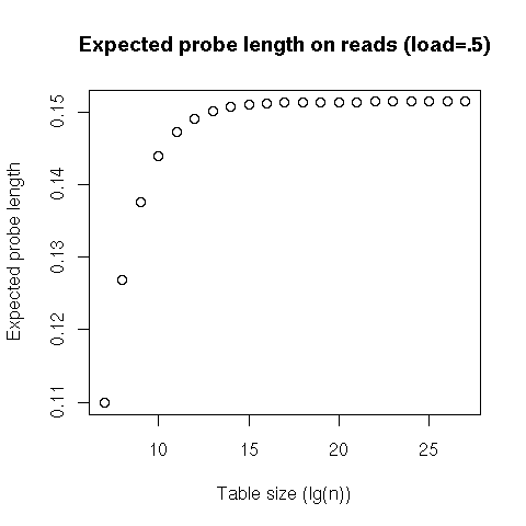
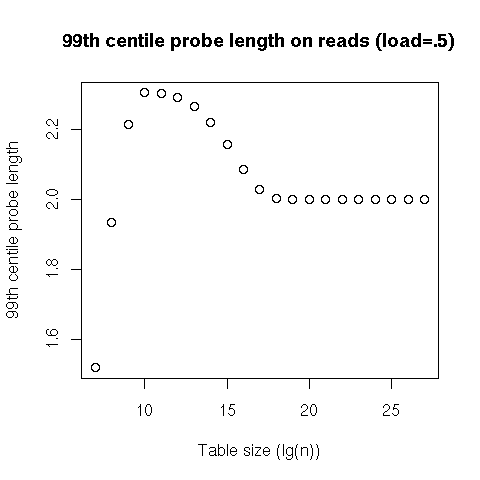
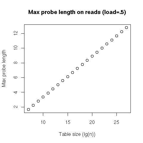
This tells us that lookups, both successful and failed, will have a constant cost on average, and even in the 99th percentile, and will usually be at worst logarithmic. Our (probabilistic) worst case is thus equivalent to the average case for search trees... except that our probes are linear, and will result in much nicer performance than a tree traversal!

That covers the cost of lookups, but inserts incur an additional cost: shifting entries to make place for the newly-inserted one. We see that the average number of entries to shift is consistently less than 1 – I don’t know what’s going on with the last two data points; it might be related to the overflow area –, and that the 99th percentile looks pretty stable, while the worst case seems, again, logarithmic.

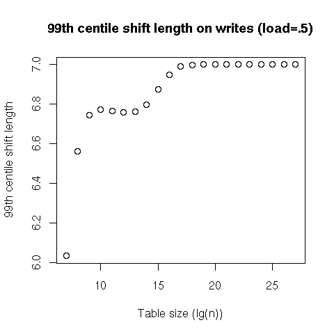
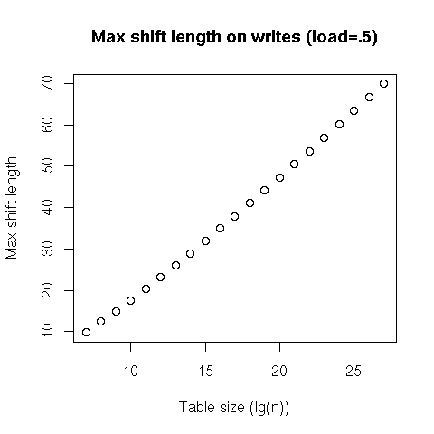
So, on average, inserts in a table at a 50% load have a constant cost; better, even the 99th percentile of insertions is still constant. Finally, the very worst case is expected to be logarithmic, but shifting contiguous entries in an array is much more efficiently executed than updating the nodes in a search tree.

3 Microbenchmarks

It looks like Robin Hood hashing with linear probing has interesting theoretical properties, but, in the end, practical performance is what matters. So, I designed a very simple microbenchmark: insert consecutive 64 bit integers in a hash table, then recover them (again, consecutively). The hash function multiplies by a randomly chosen 64 bit integer, (almost) modulo 2⁶⁴- 1. Keys and values are 64 bit integers, and there are 30 ⋅ 2¹⁷ such entries (the hash tables are preallocated to fit that many entries with the target load factor). Finally, this was executed on my 2.8 GHz X5660.

Tons of things are wrong with this setup, but I really wanted to isolate the cost of insertions and lookups, without polluting the accesses. In particular, I’m relying on the hash function to scatter the accesses around.

I’ve been using Google’s dense_hash_map as my go-to hash table for a while, so I tried and compare it with Robin Hood linear probing. dense_hash_map is an open addressing table with quadratic probing and a (default) target load factor of 50%. On the microbenchmark, inserts and lookups show a strongly bimodal distribution, with 32 cycles for ≈ 24% of inserts, and 36 c for the rest (and a bit less than 1% of outliers). Lookups, on the other hand, are evenly split between 24 c and 28 c.

My implementation of Robin Hood hashing stores the hash values alongside the keys and values. Since dense_hash_map uses a load factor of 50% by default, I went with 75% in order to have comparable space overhead. On the microbenchmark, I found that inserts also show a strong bimodal distribution, with 24 cycles ≈ 74% of the time, 28 c ≈ 25% of the time, and around 1.5 % for the rest (including ≈ 0.3% for 32 c and 36 c). Finally, almost 100% of lookups took 24 c.

Overall, it seems that both insertions and lookups in Robin Hood linear probing can be consistently faster than with quadratic probing.

4 Conclusion

I started looking at better hash tables some time ago (more than two years), and, finally, I think there’s something that’s simple and elegant, while providing exciting performance guarantees. Robin Hood linear probing preserves the nice access patterns of linear probing, on both lookups and insertions, but also avoids clustering issues; in fact, it seems to offer constant time lookups and inserts with a good probability, with logarithmic (probabilistic) worst case, even with a load factor of 75%. Also, interestingly, the layout of the table is completely independent of the order in which entries were inserted.

The theoretical performance isn’t as good as that of 2-left or cuckoo hashing. However, these two hashing schemes do not fare very well on modern commercial processors: two uncorrelated accesses can be more expensive than a surprisingly long linear search. In the end, even the worst case for Robin Hood linear probing is pretty good (logarithmic) and comparable to that of useful dictionaries like balanced search trees... and practical performance advantages like sequential access patterns look like they more than compensate the difference.

There’s one thing that I would like to see fixed with Robin Hood linear probing: it seems much harder to allow lock-free concurrent writes to it than with regular “First-come, first-served” linear probing.

Finally, there’s only one very stupid microbenchmark in this post. If you try to implement Robin Hood linear probing (after all, it’s only a couple lines of code added to a regular linear probing), I’d love to see follow-ups or even just short emails on its practical performance.