Paul Khuong mostly on Lisp

Part of what makes SBCL’s static analyses powerful is their flow-sensitivity: the system can express the fact that something is true only in one of the branches of a conditional. At the heart of that capability are sets of constraints that represent that knowledge; e.g. (eql x y) to assert that x and y hold the same value in a given branch.

Until September 2008, we implemented these sets as specialised hash tables. In commit 1.0.20.4, Richard M. Kreuter replaced the hash tables with bit vectors. On most workloads, the change was beneficial, if only because the compiler now spends less time in GC. However, in some cases (I would expect, with a large number of variables and conditional branches), users have reported severe performance regressions (e.g. https://bugs.launchpad.net/sbcl/+bug/394206), regarding not only compilation times, but also memory usage.

Exploring alternative representations for constraint sets (consets) looks like good way to get started with SBCL: it’s interesting as a data structure challenge, involves “real world” engineering trade-offs, and will have an immediate observable impact on the performance of the compiler. I’ve said as much before. Maybe this post will spur some interest.

As a first step, I instrumented the conset implementation to output some profiling information on each operation: the size of the constraint universe (approximately, the number of unique constraints in the compilation unit), and, for each conset argument, the size of the bit vector and the size of the set. I’m only using a random sample of ≈ 1% of the output from a full SBCL build.

Before graphing out histograms for the population and size of the consets, I counted the operations that were actually performed to see what was important:

All the operations should be obvious, except maybe do, which iterates over the constraints in the set, do-intersect, which iterates over the intersection of two sets, and empty, which tests for emptiness.

Of the 53% calls to member, 38% come from do-intersect, and another 14% from adjoin. There are actually very few calls to member per se. A large number of the calls to member returned T: 29%. That’s unfortunate, since failure is much easier to fast path. do is also slightly over-represented, since do-intersect also count as calls to do.

Graphs galore

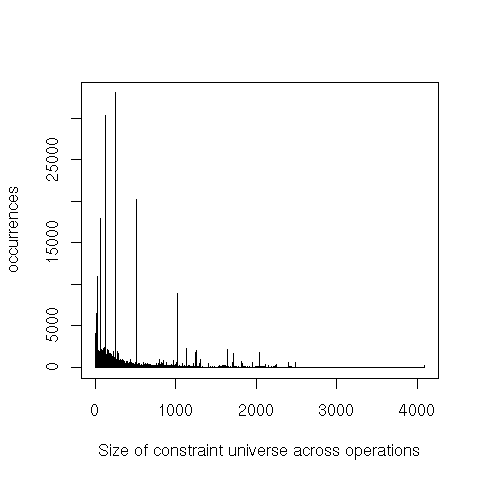
The spikes are powers of 2, and the last non-zero value is 4096. Kreuter reported that the largest universe he’d seen was 8k elements in an email. We don’t really have to worry about enormous universes except to avoid disastrous blow-ups.

We can also see that the representation as bitvector isn’t very dense. However, keep in mind that a bit is much smaller than a word. It takes very sparse sets for alternatives such as hash tables to save space.

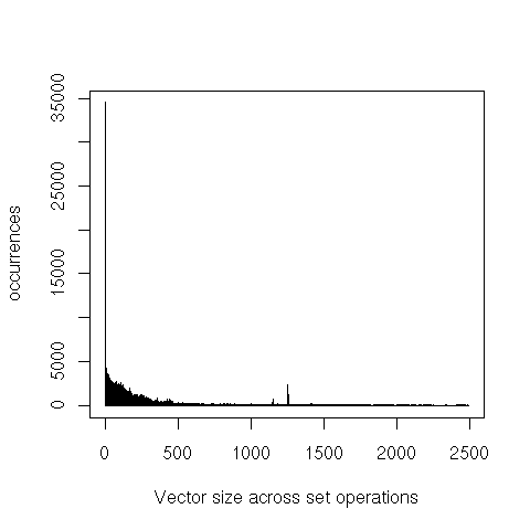
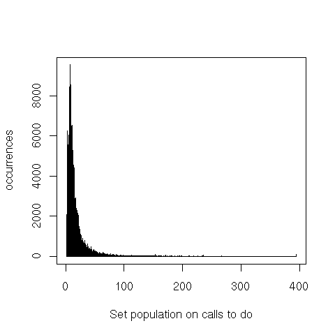
The very long tails here means that while there are some fairly large consets, the vast majority of the operations only touch sets that have less than a half dozen elements.

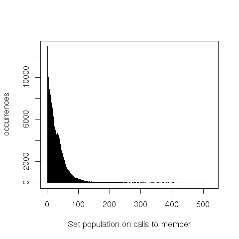
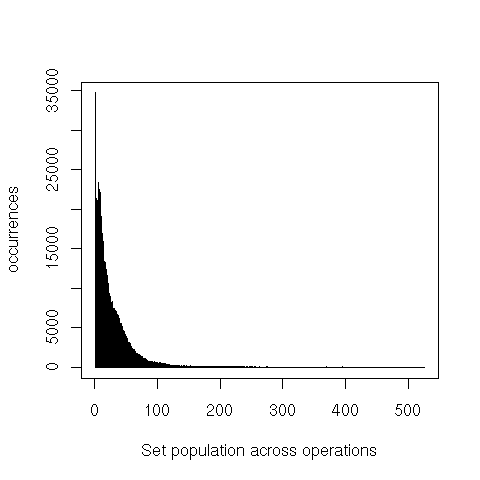
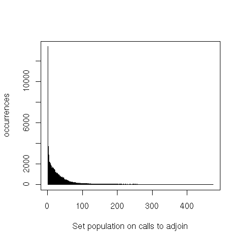
That’s also true for calls to member, but even more for adjoin and empty.

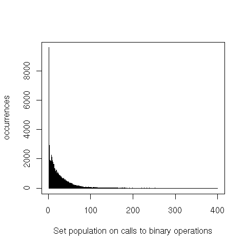
The profile for binary operations (union, intersection, difference and equal) is very similar to that of adjoin. In detail, we have:

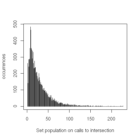
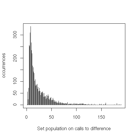
equal only shows a heavier tail. intersection and difference, however, both peak around 20 elements, instead of 1 to 3. Finally, we can see that union is pretty much a non-issue.

It’s also interesting to see the difference between the size of the largest and smallest argument for binary operations.

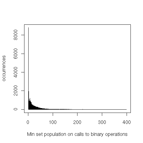
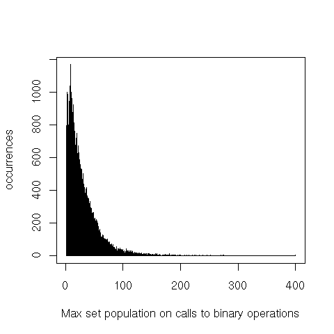
The heavier tails on binary operations probably come from the large arguments, while the smaller arguments seem to follow the overall distribution.

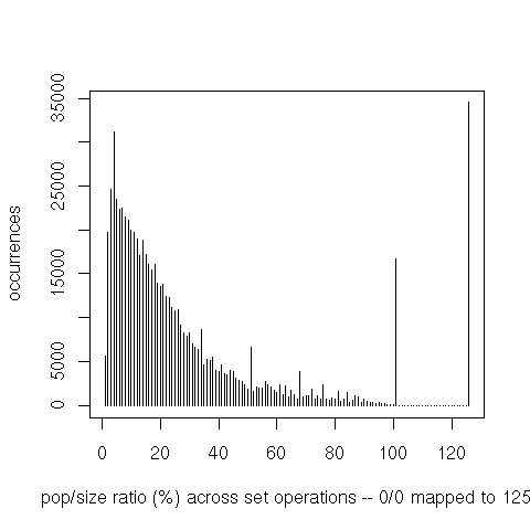
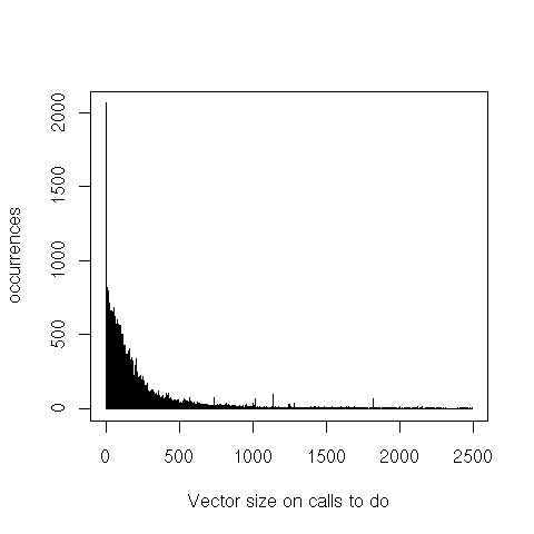
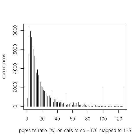
Finally, iteration through the set’s elements (do or do-intersect) is interesting because the ratio between the set’s population and the bit vector’s size is a good indicator of that operation’s performance. For do-intersect only the set that’s iterated over is counted (not the one on which member tests are then executed).

Making sense of the data

I’m not sure what information we can extract from this data, and especially not how to extrapolate to the cases reported by users who experience serious regressions.

One obvious way to speed do up is to work with vectors of fixnum or machine words, and do the rest ourselves. That would help with long spans of 0s, and would simplify the inner loop. We could do something similar for empty for implementations that don’t special-case FIND on bit-vectors (e.g. SBCL).

This does nothing to reduce memory usage. We probably want to switch to another representation for really sparse sets, a hash table or a (sorted) vector. But, if we do that, we run the risk of switching to a sparse implementation only because we have constraints with very high and very low indices, but nothing in the middle. A fat and shallow (two-level?) tree would help avoid that situation, and let us choose locally between a few representations.