In which a Lisp hacker exhibits his ignorance of applied mathematics ;)
Linear programming (LP) is awesome. I based my PhD work on solving LPs with millions of variables and constraints… instead of integer programs a couple orders of magnitude smaller. However, writing LP solvers is an art that should probably be left to experts, or to those willing to dedicate a couple years to becoming one.
That being said, if one must write their own, an interior point method (IPM) is probably the best approach. This post walks through the development of a primal affine scaling method; it doesn’t guarantee state-of-the-art practical or theoretical efficiency (it’s not even polynomial time), but is simple and easy to understand.
I think interior point methods suffer from an undeserved bad reputation: they only seem complicated compared to the nice combinatorial Simplex method. That would explain why I regularly (once or twice a year) see hackers implement a (classic!) simplex method, but rarely IPMs.
The problem is that simplex only works because world-class
implementations are marvels of engineering: it’s almost like their
performance is in spite of the algorithm, only thanks to
coder-centuries of effort. Worse, textbooks usually present the
classic simplex method (the dark force behind simplex tableaux) so
that’s what unsuspecting hackers implement. Pretty much no one uses
that method: it’s slow and doesn’t really exploit sparsity (the fact
that each constraint tends to only involve a few variables). Avoiding
the trap of the classic simplex is only the first step. Factorising
the basis — and updating the factors — is essential for efficient
revised simplex methods, and some clever tricks really help in
practice (packages like
LUSOL mostly
take care of that); pivot selection (pricing) is fiddly but has a huge
impact on the number of iterations — never mind degeneracy, which
complicates everything; and all that must be balanced with minimising
work per iteration (which explains the edge of dual simplex: there’s
no primal analogue to devex normalised dual steepest edge
pricing). There’s also presolving and crash basis construction, which
can simplify a problem so much that it’s solved without any simplex
pivot. Despite all this sophistication, only
recent theoretical advances
protect against instances going exponential.
Sidenote: Vasek Chvatal’s Linear Programming takes a view that’s closer to the revised simplex algorithm and seems more enlightening to me. Also, it’s been a while since I read about pricing in the simplex, but the dual simplex definitely has a computational edge for obscure reasons; this dissertation might have interesting details.
There’s also the learning angle. My perspective is biased (I’ve been swimming in this for 5+ years), but I’d say that implementing IPMs teaches a lot more optimisation theory than implementing simplex methods. The latter are mostly engineering hacks, and relying on tableaux or bases to understand duality is a liability for large scale optimisation.
I hope to show that IPMs are the better choice, with respect to both the performance of naïve implementations and the insights gained by coding them, by deriving a decent implementation from an intuitive starting point.
Affine scaling in 30 minutes
I’ll solve linear problems of the form \(\min\sb{x} cx\) subject to \(Ax = b\) \(l \leq x \leq u.\)
I will assume that we already have a feasible point that is strictly inside the box \([l, u]\) and that A has full row rank. Full rank doesn’t always pan out in practice, but that’s a topic for another day.
If it weren’t for the box constraint on x, we would be minimising a smooth function subject to affine equalities. We could then easily find a feasible descent direction by projecting \(-c\) (the opposite of the gradient) in the nullspace of A, i.e., by solving the linear equality-constrained least squares \(\min\sb{d} \|(-c)-d\|\sb{2}\) subject to \(Ad = 0,\) e.g. with LAPACK’s xGGLSE.
The problem with this direction is that it doesn’t take into account the box constraints. Once some component of x is at its bound, we can’t move past that wall, so we should try to avoid getting too close to any bound.
Interior point methods add a logarithmic penalty on the distance between x and its bounds; (the gradient of) the objective function then reflects how close each component of x is to its lower or upper bound. As long as x isn’t directly on the border of the box, we’ll be able to make a non-trivial step forward without getting too close to that border.
There’s a similar interpretation for simpler primal affine scaling methods we’ll implement here, but I prefer the original explanation. These methods rescale the space in which we solve for d so that x is always far from its bounds; rescaling the direction back in the original space means that we’ll tend to move more quickly along coordinates that are far from their bounds, and less for those close to either bound. As long as we’re strictly inside the box, the transformation is meaningful and invertible.
It’s a primal method because we only manipulate primal variables; dual methods instead work with the dual variables associated with the linear constraints. Primal-dual methods work on both sets of variables at once.
This sketch might be useful. x is close to the left-hand side bound, and, after projection in the nullspace, d quickly hits the border. With scaling, d is more vertical, and this carries to the unscaled direction.
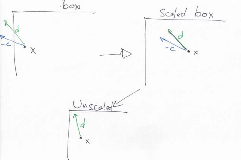
The descent direction may naturally guide us away from a close-by bound; scaling is then useless. However, each jump away from that bound makes the next longer, and such situations resolve themselves after a couple iterations.
Formally, let \(s = \min\\{x-l, u-x\\} > 0\) be the slack vector (computed element wise) for the distance from x to its bounds. We’ll just scale d and c elementwise by S (S is the diagonal matrix with the elements of s on its diagonal). The scaled least square system is \(\min\sb{d\sb{s}} \|(-Sc)-d\sb{s}\|\) subject to \(ASd\sb{s} = 0.\)
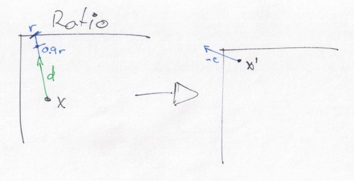
Now that we have a descent direction \(d=Sd\sb{s}\), we only have to decide how far along to go in that direction. We determine the limit, r, with a ratio test. For each coordinate, look at \(d\sb{i}\): if it’s zero, this coordinate doesn’t affect the limit; if it’s negative, the limit must be at most \((l-x)\sb{i}/d\sb{i}\); if it’s positive, the limit is at most \((u-x)\sb{i}/d\sb{i}\). We then take the minimum of these ratios.
If the minimum doesn’t exist (i.e., \(r=\infty\)), the problem is unbounded.
Otherwise, we could go up to \(x+rd\) to improve the solution while maintaining feasibility. However, we want to stay strictly inside the feasible space: once we hit a bound, we’re stuck there. That’s why we instead take a slightly smaller step, e.g., \(0.9r\).
This drawing shows what’s going on: given d, r takes us exactly to
the edge, so we take a slightly shorter step. The new solution is
still strictly feasible, but has a better objective value than the previous
one. In this case, we’re lucky and the new iterate \(x\sp{\prime}\)
is more isotropic than the previous one; usually, we slide closer
to the edge, only less so than without scaling.
We then solve the constrained least squares system again, with a new value for S.
Finding a feasible solution
I assumed that x is a strictly feasible (i.e., interior) solution: it satisfies the equality constraint \(Ax=b\) and is strictly inside its box \([l, u]\). That’s not always easy to achieve; in theory, finding a feasible solution is as hard as optimising a linear program.
I’ll now assume that x is strictly inside its box and repair it toward feasibility, again with a scaled least squares solution. This time, we’re looking for the least norm (the system is underdetermined) solution of \(Ad = (b - Ax).\)
We rescale the norm to penalise movements in coordinates that are already close to their bound by instead solving \(ASd\sb{s} = (b - Ax),\) for example with xGELSD.
If we move in direction \(Sd\sb{s}\) with step \(r=1\), we’ll satisfy the equality exactly. Again, we must also take the box into account, and perform a ratio test to determine the step size; if \(0.9r > 1\), we instead set \(r=1/0.9\) and the result is a strictly feasible solution.
An initial implementation
I uploaded some hacktastic CL to github. The initial affine scaling method corresponds to this commit. The outer loop looks at the residual \(Ax-b\) to determine whether to run a repair (feasibility) or optimisation iteration.
The code depends on a few libraries for the MPS parser and on matlisp, and isn’t even ASDF-loadable; I just saved and committed whatever I defined in the REPL.
This commit depends on a patch to matlisp’s src/lapack.lisp (and to
packages.lisp to export lapack:dgglse):
1 2 3 4 5 6 7 8 9 10 11 12 13 14 15 16 17 18 19 20 21 22 23 24 25 26 | |
1 2 3 4 5 6 7 8 | |
MPS is a very old (punchcard-oriented) format to describe linear and
mixed integer programs. The parser mostly works (the format isn’t
very well specified), and standard-form.lisp converts everything to
our standard form with equality constraints and a box around decision
variables.
I will test the code on a couple LPs from netlib, a classic instance set (I think the tarball in CUTEr is OK).
AFIRO is a tiny LP (32 variables by 28 constraints, 88 nonzeros). Good news: the program works on this trivial instance and finds the optimum (the relative difference with the reference value is 7e-6). The first four “repair” iterations find a feasible solutions, and 11 more iterations eventually get to the optimum.
1 2 3 4 5 6 7 8 9 10 11 12 13 14 15 16 17 18 19 20 21 22 23 24 25 26 27 28 29 30 31 32 33 34 35 36 | |
I also tested on ADLITTLE, another tiny instance (97x57, 465 nz): 48 iterations, 0.37 seconds total.
AGG is more interesting, at 163x489 and 2541 nz; that one took 156 iterations and 80 seconds (130% CPU, thanks to Apple’s parallel BLAS). Finally, FIT1D is challenging, at 1026x25 and 14430 nz; that one took 100 seconds and the final objective value was off by .5%.
All these instances are solved in a fraction of a second by state-of-the-art solvers. The next steps will get us closer to a decent implementation.
First, simplify the linear algebra
The initial implementation resorted to DGGLSE for all least squares solves. That function is much too general.
I changed the repair phase’s least squares to a GELSY (GELSD isn’t nicely wrapped in matlisp yet).
We can do the same for the optimisation phase’s constrained least squares. Some doodling around with Lagrange multipliers shows that the solution of \(\min\sb{x} \|x-c\|\sb{2}\sp{2}\) subject to \(Ax = 0\) is \(x = A\sp{t}(AA\sp{t})\sp{-1}Ac - c.\)
This is a series of matrix-vector multiplications and a single linear solve, which I perform with GELSY for now: we need the numerical stability because, when we’re close to optimality, the system is really badly conditioned and regular linear solves just crash.
Both linear algebra microoptimisations are in this commit.
ADLITTLE becomes about five times faster, and FIT1D now runs in 2.9 seconds (instead of 100), but AGG eventually fails to make progress: we still have problems with numerical stability.
Now, the magic sauce
Our numerical issues aren’t surprising: we work with a scaled matrix \(AS\), where the diagonal of \(S\) reflects how close \(x\) is to its bounds. As we get closer to an optimal solution, some of \(x\) will converge to the bounds, and some to a value in-between: the limit is a basic solution. We then take this badly conditioned matrix and multiply it by its own transpose, which squares the condition number! It’s a wonder that we can get any useful bit from our linear solves.
There’s a way out: the normal matrix \(AA\sp{t}\) is not only symmetric, but also positive (semi)definite (the full rank assumption isn’t always satisfied in practice). This means we can go for a Cholesky \(LL\sp{t}\) (or \(LDL\sp{t}\)) factorisation.
We’re lucky: it turns out that Cholesky factorisation reacts to our badly conditioned matrix in a way that is safe for Newton steps in IPMs (for reasons I totally don’t understand). It also works for us. I guess the intuition is that the bad conditioning stems from our scaling term. When we go back in the unscaled space, rounding errors have accumulated exactly in the components that are reduced into nothingness.
I used Cholesky factorisation with LAPACK’s DPOTRF and DPOTRS for the optimisation projection, and for repair iterations as well.
LAPACK’s factorisation may fail on semidefinite matrices; I call out to GELSY when this happens.
To my eyes, this yields the first decent commit.
The result terminates even closer to optimum, more quickly. AGG stops after 168 iterations, in 26 seconds, and everything else is slightly quicker than before.
Icing on the cake
I think the code is finally usable: the key was to reduce everything to PD (positive definite) solves and Cholesky factorisation. So far, we’ve been doing dense linear algebra with BLAS and LAPACK and benefitted from our platform’s tuned and parallel code. For small (up to a hundred or so constraints and variables) or dense instances, this is a good simple implementation.
We’ll now get a 10-100x speedup on practical instances. I already noted, en passant, that linear programs in the wild tend to be very sparse. This is certainly true of our four test instances: their nonzero density is around 1% or less. Larger instances tend to be even sparser.
There’s been a lot of work on sparse PD solvers. Direct sparse linear solvers is another complex area that I don’t think should be approached lightly: expensive supercomputers have been solving sparse PD linear systems for a couple decades, and there’s some really crazy code around. I’ve read reports that, with appropriate blocking and vectorisation, a sparse matrix can be factored to disk at 80% peak FLOP/s. If you’re into that, I’m told there are nice introductions, like Tim Davis’s book, which covers a didactical yet useful implementation of sparse Cholesky in 2000 LOC.
I decided to go with CHOLMOD from
SuiteSparse, a
mixed GPL/LGPL library. CHOLMOD implements state of the art methods:
when all its dependencies are available, it exposes parallelisation
and vectorisation opportunities to the BLAS (thanks to permutations
computed, e.g., by METIS) and exploits Intel’s TBB and Nvidia’s CUDA.
It’s also well designed for embedding in other programs; for example,
it won’t abort(3) on error (I’m looking at you, LLVM), and includes
data checking/printing routines that help detect FFI issues. Its
interface even helps you find memory leaks! Overall, it’s a really
refreshing experience compared to other academic code, and I wish all
libraries were this well thought out.
I built only the barest version on my Mac and linked it with a
wrapper
to help
my bindings.
I had to build the dynamic library with -Wl,-all_load on OS X to
preserve symbols that only appear in archives; -Wl,--whole-archive
should do it for gnu ld. (I also bound a lot of functions that I
don’t use: I was paying more attention to the TV at the time.)
CHOLMOD includes functions to simultaneously multiply a sparse matrix with
its transpose and factorise the result.
Function solve-dense
shows how I use it to solve a dense PD system. It’s a three-step
process:
- Analyse the nonzero pattern of the constraint matrix to determine an elimination order (trivial for a dense matrix);
- Compute the normal matrix and factor it according to the analysis stored in the factor struct;
- Solve for that factorisation.
This is really stupid: I’m not even dropping zero entries in the dense matrix. Yet, it suffices to speed up AGG from 26 to 14 seconds!
It’s clear that we need to preserve the constraint matrix A in a sparse format. CHOLMOD has a function to translate from the trivial triplet representation (one vector of row indices, another of column indices, and another of values) to the more widely used compressed representation. Instances in our standard form already represent the constraint matrix as a vector of triplets. We only have to copy from CL to a CHOLMOD triplet struct to exploit sparsity in Cholesky solves and in matrix-vector multiplications.
We now solve AGG in 0.83 seconds and FIT1D in 0.95. I think we can expect runtimes of one second or less for instances up to ~200x200. Better, we can finally hope to solve respectable LPs, like FIT2D (10500x26, 138018 nz, 2.3 s) or FIT1P (1677x628, 10894 nz, 14 s).
Finishing touches
Our normal matrix \(ASS\sp{t}A\sp{t}\) always has the same pattern (nonzero locations): we only change the scaling diagonals in the middle. Sparse solvers separate the analysis and factorisation steps for exactly such situations. When we solve a lot of systems with the same pattern, it makes sense to spend a lot of time on a one-time analysis that we then reuse at each iteration: fancy analysis routines generate factors that take up less space and need fewer FLOPs to build.
I do that here. Our less tiny instances are almost twice as fast. We solve FIT1P in 8 seconds now, and even FIT2P (13525x3001, 60784 nz) in 200 seconds.
I then made some microoptimisation to reuse storage.
Finally, I added steps that push the current solution away from close-by bounds. These centering steps help subsequent iterations make longer jumps toward optimality
The last two changes shave a couple more seconds on large instances and gets closer to optimality on nastier ones.
Not quite the end
I hope I managed to communicate the intuition behind primal affine scaling methods, and that the walkthrough helped map that intuition to a sparse implementation. I also realise that the code isn’t pretty: I wrote it during a short marathon and tried to only make incremental changes. Still, the algorithm should be more or less usable for small instances; more than a naïve simplex method, anyway.
That’s particularly true on multicore machines. Parallelising simplex methods has been an area of slow research for a couple decades; the best work I’ve seen so far takes a huge hit by reverting to the classic algorithm and hopes that parallelisation can compensate for that initial 10-1000x slowdown. In contrast, even our sparse method is already parallel: CHOLMOD automatically vectorises, parallelises, and offloads work to the GPU.
I’ll try to code a sparse primal-dual affine scaling method from scratch soon. Primal-dual methods usually work better than pure primal (or dual) methods and I find their theory interesting (if a bit complicated).
If you liked this post, you might be interested in Stephen Boyd’s Convex optimisation course. He’s offering it online this winter, starting January 21st.